Background
The project studies a Magic 8 Ball simulator that combines particle-based fluid motion, a spherical container, and a rigid die that moves through and reacts to the fluid. The simulator has a reference CPU implementation as well as a CUDA implementation of the same timestep pipeline. Both versions produce a binary SIM2 frame stream that encodes particle positions, particle densities, and die pose data. Then, a simple visualizer reads the stream to render the fluid, ghost boundary particles, and die motion.
Initialization.
The simulation occurs within a sphere of radius SPHERE_R. Fluid particles are initialized within this sphere using Poisson-disk sampling. We basically just place a particle and then randomly place another particle a certain distance apart. This distance is computed to reach the target particle count within the total volume of the sphere. The reason for this method of sampling is that it breaks any artifacts introduced by symmetry. After the sampler goes through and places all the particles, the algorithm computes a per-particle mass based on the rest density and the fluid volume.
The die is modeled as a rigid cube with position, linear velocity, angular velocity, quaternion orientation, mass, and inertia. The mass is chosen based on the fluid density and the die volume such that it is neutrally buoyant within the fluid.
The state uses a structure of arrays layout where we have a structure that stores contiguous arrays such as $ pos_x$, $ pos_y$, density, and pressure. This allows us to store each particle's statistics that we need in order to do all of our computations in a way that is cache-friendly as well as better for GPU memory locality. The one complication is that we have double-buffered velocities with ping-pong arrays in which we read from one buffer while writing to the other and then swap buffers every time step. This prevents a timestep from using stale or inconsistent information.
Spatial Neighborhoods
The most expensive part of this simulation is to figure out which particles neighbor each particle at each time step. The naive approach compares all particles against all others, which scales poorly. The simulator instead uses a uniform spatial partition with a cell size equal to the smoothing radius. Each particle is then assigned to a grid cell, and particles are grouped by cell. Then, each particle only checks its own cell and the 26 adjacent cells, as any particle within radius H must lie in a neighboring cell (as each grid cell is sized to be exactly one radius).
We construct this neighbor list (which is capped at MAX_NEIGHBORS for memory use and density simplicity) and then use it to compute all the sph things.
SPH Density, Pressure, and Forces
The first step of our per-step method's physics steps is to get our density, pressure, and forces. We do this by weighting nearby particles with smoothing kernels. Our simulator has 3 kernels, each of which is used for a different operator. We use the Poly6 kernel to estimate density because it is smooth close to 0 distance and can be evaluated from a squared distance. We use the spiky kernel gradient for pressure forces because it produces useful non-zero pressure gradients between close particles. We use a viscosity kernel Laplacian to diffuse velocity differences between neighbors.
Concretely, for each fluid particle $i$, density is computed by summing the mass-weighted Poly6 contribution of every neighbor $j$ within radius $H$, plus the particle's self contribution:
\[
\rho_i = m_i W(0) + \sum_j m_j W(\lVert x_i - x_j \rVert^2).
\]
The result is clamped to a small positive floor to avoid division by zero. Pressure is then computed with a Tait-style equation of state:
\[
p_i = k \left(\left(\frac{\rho_i}{\rho_0}\right)^7 - 1\right),
\]
where $k$ is the stiffness parameter and $\rho_0$ is the rest density. Negative pressures are clamped to zero, so the pressure term acts as a restoring force when local density rises above the target value.
Then, to do force accumulation, we combine pressure, viscosity, gravity, and velocity smoothing. The pressure term has a symmetric expression that involves both particles' pressure and densities, which prevents any one particle's state from dominating an interaction. The viscosity term is used to damp relative velocity between neighboring particles. Gravity contributes a constant body force. Then, XSPH keeps fluid motion smooth by making particles follow their neighbors, while ignoring the "ghost" particles used for walls.
Fluid-Die Coupling
The die interacts with the fluid through contact and drag. The simulator handles this by, on each step, seeing if particles are within the die's contact margin and computing a contact force along the die surface normal. This term is essentially a spring where a deeper penetration will result in a larger restoring force.
Then, we observe the relative difference in velocity between the fluid particles and the die, which allows us to calculate contact force minus drag, and then we can provide this to the fluid and give the die a reaction force. This reaction force from each particle is accumulated into the die's net force, and we use each particle's offset and cross it with the reaction force in order to give a per-particle torque contribution, which we use to sum together a total torque on the die. All of this leads to a two-way coupling where the fluid pushes the die, and the die pushes the fluid.
Timestep scaling and Integration
The simulator uses explicit integration, so the timestep size is very important for stability. Instead of advancing with a constant time step, the simulation computes several candidate limits and finds the smallest value within configured bounds. There is an acoustic limit that accounts for the pressure wave speed from the equation of speed. There is a force limit that reacts to large accelerations. There is finally a viscous limit that accounts for diffusion. The selected value is then clamped between DT_MIN and DT_MAX.
After we know the exact forces and timesteps, we have each fluid particle update velocity from acceleration and position from velocity. We then use a spherical boundary pass to ensure that each particle remains within the sphere itself. If it is, we reflect its normal velocity across the wall and dampen tangential velocity according to friction. Finally, we integrate the die with its accumulated force and torque and update the orientation and position. We then clamp the die inside the spherical container.
Pipeline
- Ghost Injection
- Spatial Hash
- Neighbor Lists
- Density
- Pressure
- Forces + XSPH
- Die Coupling
- Adaptive $\Delta t$
- Fluid Integrate
- Boundary + Die Update
CPU pipeline
Pipeline information
This order matters. Pressure depends on density; forces depend on pressure, density, and neighbors; integration depends on forces and the selected timestep; the die update depends on accumulated reactions from many particles. The main performance cost comes from operations that repeat across all particles and their neighbors: neighbor construction, density evaluation, force evaluation, and global reductions for timestep selection. These costs make the project a strong candidate for GPU parallelization because most particle updates are independent once the required input arrays for a stage are available.
Workload breakdown
Each step of the pipeline is dependent on the prior step of the pipeline because it uses values computed in the prior stage. However, each stage itself exposes significant parallelizing capabilities as it performs essentially the same computation on a huge number of particles. It is therefore data parallel and amenable to SIMD and SIMT execution. It is especially amenable to SIMT execution as the operations themselves are fairly simple. Locality exists due to spatial locality of particles where particles that affect each other are "close" to each other in the sim and therefore can be stored close to each other in memory. Temporal locality across time steps exists because the adaptive dt prevents particles from moving excessively between timesteps.
Approach
The CUDA implementation parallelizes the same simulation model by keeping the full simulation state on the GPU and decomposing each timestep into kernels that operate over particles, cells, or reductions. The final goal is to preserve the semantics of the CPU pipeline while replacing the serial loops with SIMT execution. Most kernels use one thread per particle. Some shared global quantities, such as the adaptive timestep and die reductions, are handled with reductions or atomic accumulation. Importantly, the only CPU <-> GPU data transfers after initialization (which is done entirely on the CPU) are to send control inputs to the GPU, and send particle information (minimum required) back to the CPU for rendering.
Initialization
This project is mostly concerned with asymptotic speedup for long-running simulations, and so we chose to exempt initialization from our GPU-acceleration efforts. The most important portion of initialization when understanding the GPU fork (which leads to longer initialization times on the GPU) is that the CPU, upon computing the full initial state, uploads it all to the GPU.
GPU State and Memory Layout
The GPU implementation mirrors the CPU structure of the array design with persistent device buffers for each of the arrays present in the CPU state. Initialization uploads the arrays once, allocates CUDA-side runtime buffers, uploads simulation parameters, and stores the die into the device's memory. After initialization, steady state behavior avoids copying the full particle state back to the host. Host-Device transfers are only used for diagnostics and control values.
Parallel Ghost maintenance
Ghost particles are rebuilt on the GPU to avoid round-tripping particle positions. The CUDA path compacts real fluid particles into the prefix of arrays, removing old ghosts. It then marks all fluid particles within one smoothing radius of the sphere wall, uses an exclusive scan to compute each new ghost's destination offset, scatters new ghost particles into the tail of the arrays, and writes the new particle count to device memory.
Parallel Spatial indexing and neighbor construction
We use spatial hashing to avoid checking every particle against every other particle every step. Since our particles are inside a small fixed sphere, we can use a fixed-length grid instead of a general hash table. Each particle is mapped to a grid cell, the cell coordinate is biased so negative positions become valid indices, and that cell index becomes the particle’s key.
On the GPU, we compute these keys in parallel, sort particles by key, and store the start/end range for each grid cell. Then each particle only searches particles in nearby cells contiguously when building its neighbor list.
We are allowed to do this because our simulation domain is bounded and known ahead of time. A normal spatial hash needs to handle large or unbounded space and hash collisions. Ours does not, so we can trade generality for speed.
Parallel Die Coupling and Reductions
We also parallelize the die coupling with one thread per particle. Each thread checks whether its particle is a real fluid particle, evaluates the die-signed distance contact condition, computes the force and drag forces when applicable, and adds the resulting fluid force to that particle. The die reaction is a shared quantity, and so we can't just use simple independent stores. So, we use block-local accumulation and global atomic additions to combine the particle reaction forces and torques into device-side die accumulators.
Adaptive time is done by having a kernel compute per block maxima for speed and acceleration, then we use a scalar reduction to combine block maxima, and then use a finalization kernel to evaluate each time step limit to get our real time step limit.
Parallel integration
Fluid integration is embarrassingly parallel once forces and timestep are known. A kernel updates velocity and position for each fluid particle using the given time step and force information. Then we have a small kernel to swap the velocity buffers. Then, finally, we have a boundary kernel check each particle against the sphere radius and apply the clamp, restitution, and damping logic as with the CPU implementation.
The rigid die update is done after the accumulation has already been loaded into device buffers. We therefore just have to use an integration kernel to apply caps, gravity, buoyancy, damping, linear and angular updates, and quaternion normalization. Then, a kernel keeps the die within the spherical container by clamping it. Although there isn't as much parallelism in these kernels as in the particle kernels, we keep them on the device to avoid unnecessary synchronization and host-device transfers during time steps.
GPU Pipeline
- Control Upload & Preprocess
- Ghost Management & $n_{total}$
- Spatial Rebuild / Reuse
- Density & Pressure
- Fluid Forces
- Die Coupling & Reductions
- Adaptive $\Delta t$ Reduction
- Integrate & Buffer Toggle
- Boundary & Rigid Update
- Advance Simulation Clock
GPU implementation flow
Orchestration Logic
The host function sim_gpu_advance acts as a high-level scheduler, orchestrating the GPU timestep through a sequence of dependent launch groups. While the ordering strictly preserves CPU dependencies, which ensures that pressure calculation follows density and integration follows force accumulation.
By offloading per-particle computation to the device, the host is freed from heavy arithmetic, focusing instead on managing constant memory uploads for controls and performing global reductions for adaptive time stepping. To maintain performance, the implementation avoids full device synchronization after every kernel launch in normal execution mode, opting for lightweight error checking unless strict debugging mode is enabled for diagnostic trace-backs.
Iterative Optimization Journey
Our first GPU-accelerated fork was done in two stages. First, we converted the compute_density, compute_pressure, compute_forces, integrate, handle_boundary functions into kernels. The speedup is attached below.
Round 1a
The speedup was incredibly modest because at every step, there was a lot of CPU-GPU data transfer. This was fixed when we moved the rest of our functions to CUDA and sought to eliminate all data transfers (more on this later). This led to a much improved speedup. We also realized while combining our code that we were having our ping ponged buffers set up to be vel[i][ping/pong] and so we flipped this so that each warp gets a contiguous block of memory to update (this was not done on the CPU as it slowed our CPU implementation).
All GPU
To note, we recorded the speedup below on the exact same code.
Bad bad bad bad bad so bad
We realized that our benchmarking metrics were introducing a lot of noise in our speedup calculations. We mainly care about how quickly we can produce new sim frames at steady state, not really how long it takes to initialize the data structures. By including initialization time in the speedup calculation, we were allowing for differences in initialization time to appear as large speedup gains, even though they were not. We saw this issue a lot when we started optimizing to the point where each step was very fast, because then any changes in initialization time represented a much larger portion of overall runtime, making the output noisier. To address this, we excluded init time from future speedup calculations, since it takes a nondeterministic amount of time (Poisson disk sampling is random), and we care more about frames per second than overall time.
| Kernel Name |
Time (%) |
Instances |
Med (ns) |
Min (ns) |
Max (ns) |
StdDev (ns) |
| kernel_build_neighbor_lists | 87.2 | 500 | 2,621,750.0 | 2,318,199 | 2,889,301 | 122,806.2 |
| kernel_compute_forces | 5.0 | 500 | 150,303.5 | 138,719 | 160,095 | 2,822.2 |
| kernel_compute_density_pressure | 1.3 | 500 | 40,543.5 | 35,425 | 50,624 | 1,448.5 |
| DeviceRadixSortDownsweepKernel | 1.2 | 1,500 | 11,712.0 | 10,784 | 22,592 | 560.3 |
| DeviceRadixSortDownsweepKernel | 1.1 | 1,000 | 16,896.0 | 16,032 | 24,800 | 384.2 |
| RadixSortScanBinsKernel | 1.0 | 2,500 | 6,368.0 | 5,599 | 17,920 | 498.6 |
| DeviceRadixSortUpsweepKernel | 0.5 | 1,500 | 4,736.0 | 3,967 | 12,544 | 444.4 |
| DeviceRadixSortUpsweepKernel | 0.4 | 1,000 | 6,304.0 | 5,472 | 19,904 | 581.9 |
| DeviceScanKernel | 0.3 | 1,000 | 4,320.0 | 3,359 | 13,568 | 502.0 |
| kernel_die_coupling | 0.2 | 500 | 4,704.0 | 3,680 | 5,728 | 206.6 |
| DeviceScanInitKernel | 0.1 | 1,000 | 2,320.0 | 1,760 | 12,224 | 555.5 |
| kernel_integrate_rigid_die | 0.1 | 500 | 3,840.0 | 3,104 | 3,936 | 80.7 |
| kernel_scatter_ghost_particles | 0.1 | 500 | 3,744.0 | 2,976 | 13,888 | 706.4 |
| kernel_integrate | 0.1 | 500 | 3,744.0 | 2,975 | 3,904 | 114.6 |
| kernel_dt_block_max | 0.1 | 500 | 3,680.0 | 2,911 | 12,992 | 431.0 |
| kernel_boundary | 0.1 | 500 | 3,393.0 | 2,624 | 3,456 | 111.7 |
| kernel_finalize_dt | 0.1 | 500 | 3,328.0 | 2,559 | 12,320 | 419.2 |
| kernel_hash_particles | 0.1 | 500 | 3,360.0 | 2,560 | 11,584 | 421.6 |
| kernel_reduce_dt_block_to_scalar | 0.1 | 500 | 3,168.0 | 2,432 | 3,328 | 77.2 |
| kernel_count_buckets | 0.1 | 500 | 3,072.0 | 2,912 | 11,296 | 368.9 |
| kernel_shake_control_preprocess | 0.1 | 500 | 3,040.0 | 2,303 | 3,776 | 98.0 |
| kernel_clamp_die_sphere | 0.1 | 500 | 2,912.0 | 2,176 | 3,136 | 98.2 |
| kernel_advance_sim_clock | 0.1 | 500 | 2,912.0 | 2,144 | 10,144 | 341.8 |
| kernel_mark_ghost_particles | 0.1 | 500 | 2,848.0 | 2,144 | 11,328 | 386.1 |
| kernel_toggle_ping | 0.1 | 500 | 2,752.0 | 2,016 | 2,816 | 54.1 |
| kernel_fill_radix_sentinels | 0.1 | 500 | 2,688.0 | 1,920 | 2,752 | 269.3 |
| kernel_write_n_total | 0.1 | 500 | 2,784.0 | 1,984 | 2,881 | 360.3 |
Kernel Execution Profiling Results
The profiling information told us that we should focus on optimizing kernel_build_neighbor_lists, since it took up 87% of the runtime. We realized that the hash-based method led to poor spatial locality as it sent contiguous memory accesses far apart from each other in location. The reason people do spatial hashing is to enforce load-balanced bins, but the nature of our sim leads to natural load balancing throughout the sphere, and so we used a simple geometric binning approach. We also discovered a lot more allocation of memory than we anticipated. Eventually, we found out that it was the Thrust sorting function we were using that was allocating buffers under the hood every time we called it. To fix this we switched over to CUB for sorting, since we were able to pre-allocate a single buffer and reuse it for every step, which significantly improved performance. These optimizations led to our speedup imrpoving from around 7× to 13×.
After profiling again, we noticed that there was a ton of data being transferred with cudaMemcpyToSymbol. Confused, we looked through our code to find any data transfers being done in the main step loop. We realized that we were passing the number of ghost particles back and forth between the CPU and GPU every step to calculate the total number of particles. We were also reducing particle forces onto the die using a partial reduction on the GPU, and then doing the final reduction on the CPU. This required that all the partial reductions be sent back to the CPU, just for a simple sum to be computed, and then to send all the data back, many times per step. This was extremely inefficient, and to fix it, we decided to keep all the sim state only on the GPU. We wanted to prevent the CPU from doing any computations if possible. We did this by replacing some of the CPU operations with 1x1 kernels that did the same thing without having to move the data. This resulted in a massive speedup, bringing us to 65×.
No more data transfer!
This was the first version of the simulator that was able to simulate particle motion at 60 Hz, which was our target for the real-time demo. However, we were not able to actually render the frames in real time, since we were still using a matplotlib-based renderer, which was too slow. So we switched to a C++ based renderer and were able to stream the sim in real time.
We then tried a few more smaller rounds of optimizations, such as reducing the number of kernel launches by consolidating neighboring kernels into larger ones, and folding the 1x1 kernels to be within other kernels, but these produced modest speedups. We realized that any significant speedup would be found in kernel_build_neighbor_lists, since that still took up around 45% of the runtime
With this in mind, we went back to build_neighbor_lists and looked for anything else we could do to squeeze out more performance. We ended up finding a small debug if statement that verified that the cell key was the same as the sorting key when building the neighbor list. This was a holdover from when we were first implementing build_neighbor_lists, and would never actually trigger under normal operation. Just by removing this redundant check, we were able to get a speedup (+20x), even though it didn't affect the algorithmic complexity at all. This brought our overall speedup to 96×.
Final speedup
Another idea we had to reduce time spent building neighbor lists was to only rebuild every k steps. We know that particles don't move much between steps (we guarantee this by reducing the $\Delta t$ based on the max particle speed. So we tested different semi-static building intervals to 2, 4, and 8 to see how much it affected performance. Unsurprisingly it had a big impact, but we were more curious how it affected correctness. If a neighboring particle moves outside of a neighboring cell without it rebuilding, then the particle interaction will be missed. We experimented with dynamic rebuilding intervals based on when particles actually leave the cell, but we found that the overhead of tracking particle position erased any gains that we would get by rebuilding less frequently.
Afterwards, we ran benchmarks on our final implementation to see the effects of each optimization.
| Implementation Variant |
Speedup |
| Semi-static neighbor rebuild, k = 8 | 1.880× |
| Neighbor lists instead of brute force searching | 1.613× |
| Semi-static neighbor rebuild, k = 4 | 1.606× |
| CUB sorting instead of Atomic add | 1.558× |
| Fused kernels | 1.481× |
| Don't transfer ntotal and die coupling reductions each step | 1.317× |
| Semi-static neighbor rebuild, k = 2 | 1.268× |
| CUB sorting instead of Thrust | 1.221× |
| Reduction in shared memory | 1.182× |
| Imprecise square root | 1.176× |
| Ping-pong major buffer | 1.140× |
| Removing inner loop check in neighbor lists | 1.115× |
Effect of each optimization sorted by effect
Results
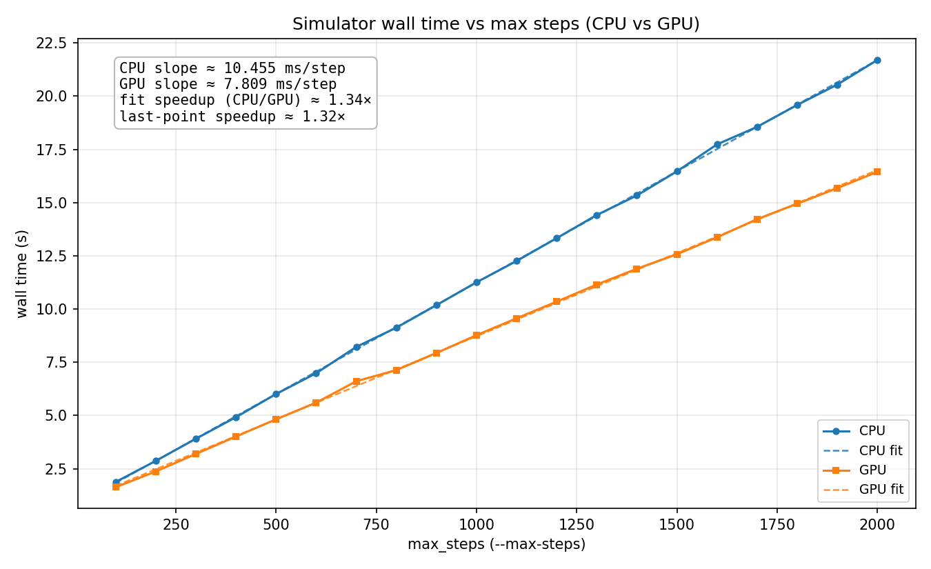
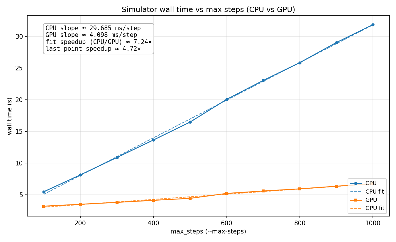
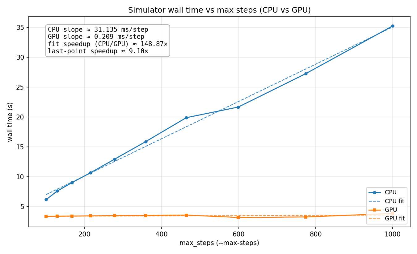
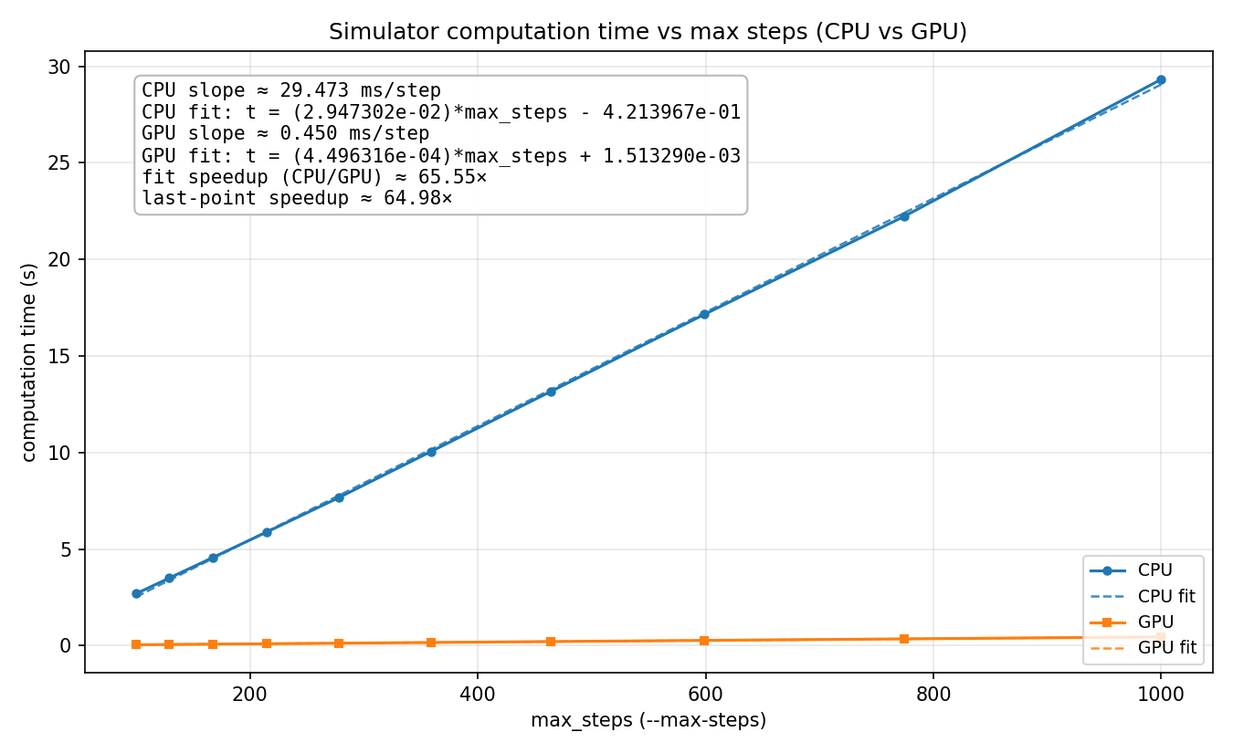
In our results we observe that running the sim for more timesteps leads to linear growth. This is to be expected as the work per time step is constant, no matter how many time steps we take.
We measured our performance with computation time (time per sim step) against a serial CPU baseline. We did not modify the CPU implementation across our various improvements so that it would remain a fair baseline. We did not consider initialization time very much since the goal of the project was to have a sim that can run in real time, and the user experience is much more affected by the smoothness and frame rate of the simulation in stead-state rather than how long it takes for the sim to start up. By virtue of maintaining a static baseline, increases in speedup are directly proportional to decreases in clock time and vice versa.
The size of our inputs were built to simulate a real 8-ball. We sized the 8 ball accordingly, and the die was also sized to approximate a real 8 ball (albeit with a cubic die). From here, we tuned our physics parameters to make the sim stable and have realistic behavior, and simply maintained these parameters while we optimized. We've attached relevant parameters below.
Smoothing and Discretization Constants
// Smoothing and discretization
constexpr float H          = 0.05f;
constexpr float PARTICLE_R = H / 2.0f;
constexpr float PARTICLE_M = 0.008f; // kg
constexpr float SPHERE_R   = 0.15f;  // inner radius of sphere
constexpr float DEFAULT_FLUID_DENSITY = 1000.0f; // kg/m^3
constexpr int   N_PARTICLES           = 3500; // target count
From this, our experiements simply ran the sim for some number of timesteps (which we swept across).
Problem Size Sweep
It is worth noting that the number of particles (3500) was chosen because that results in the most stable and realistic looking sim, not because it gave the best speedup (it doesn't). Our speedup would be much greater if we boosted the number of particles in order to get better hardware utilization on the GPU and a higher proportion of parallelizable work. When we tested our GPU implementation with higher particle counts we saw that the speedup is linear with the number of particles.
On the matter of the execution profile, our intiialziation time for the CPU with our default problem size is usually around 2.37 seconds, and for the GPU it is around 2.94 seconds. The extra GPU time is spent copying the buffers onto the GPU.
From here, we simply run a series of kernels one after the other, so the rest of the algorithm's execution time can be simply broken down by the nsys profile.
| Kernel Name |
Time (%) |
Instances |
Med (ns) |
Min (ns) |
Max (ns) |
StdDev (ns) |
| kernel_build_neighbor_lists | 36.5 | 500 | 151,120.0 | 135,808 | 173,665 | 6,041.3 |
| kernel_compute_forces | 29.9 | 500 | 124,544.0 | 118,369 | 127,680 | 1,396.8 |
| kernel_compute_density_pressure | 5.6 | 500 | 23,328.0 | 21,056 | 27,584 | 761.8 |
| DeviceRadixSortDownsweepKernel | 5.4 | 1,000 | 11,200.0 | 10,176 | 12,224 | 457.3 |
| RadixSortScanBinsKernel | 2.9 | 1,000 | 6,016.0 | 5,568 | 6,528 | 312.9 |
| DeviceRadixSortUpsweepKernel | 2.1 | 1,000 | 4,448.0 | 3,904 | 9,952 | 372.5 |
| DeviceScanKernel | 2.0 | 1,000 | 4,129.0 | 3,392 | 12,864 | 304.0 |
| kernel_die_coupling | 1.6 | 500 | 6,560.0 | 3,488 | 10,880 | 973.7 |
| kernel_compact_real_fluid_to_prefix | 1.4 | 500 | 5,728.0 | 4,928 | 7,424 | 127.0 |
| kernel_reorder_particle_arrays | 1.3 | 500 | 5,584.0 | 4,927 | 7,488 | 349.5 |
| kernel_integrate_rigid_die | 1.2 | 500 | 4,992.0 | 4,192 | 5,856 | 115.7 |
| kernel_scatter_ghost_particles | 1.2 | 500 | 4,928.0 | 4,096 | 5,057 | 142.5 |
| DeviceScanInitKernel | 1.1 | 1,000 | 2,528.0 | 1,792 | 2,624 | 289.6 |
| kernel_integrate | 1.0 | 500 | 4,000.0 | 3,200 | 4,065 | 108.2 |
| kernel_dt_block_max | 0.9 | 500 | 3,967.0 | 3,168 | 4,064 | 103.2 |
| kernel_reduce_dt_and_finalize | 0.9 | 500 | 3,744.0 | 2,944 | 3,777 | 111.6 |
| kernel_boundary | 0.9 | 500 | 3,648.0 | 2,848 | 3,808 | 97.1 |
| kernel_hash_particles | 0.8 | 500 | 3,296.0 | 2,496 | 3,744 | 114.7 |
| kernel_fill_cell_ranges | 0.7 | 500 | 3,104.0 | 2,304 | 3,168 | 187.5 |
| kernel_fill_fluid_compact_stencil | 0.7 | 500 | 2,848.0 | 2,080 | 3,296 | 84.3 |
| kernel_mark_ghost_particles | 0.7 | 500 | 2,848.0 | 2,048 | 2,976 | 297.2 |
| kernel_toggle_ping | 0.6 | 500 | 2,752.0 | 1,952 | 2,816 | 205.6 |
| kernel_reset_sorted_id | 0.6 | 500 | 2,304.0 | 1,888 | 2,784 | 281.5 |
| kernel_init_particle_ids | 0.0 | 1 | 2,144.0 | 2,144 | 2,144 | 0.0 |
Kernel Execution Profiling Results After Optimization
The final profiling table shows that particle-particle (kernel_build_neighbor_lists and kernel_compute_forces) interaction still takes up the majority of runtime.
| Metric |
Unit |
Minimum |
Maximum |
Average |
| Kernel time | μs | 165.536 | 166.688 | 166.112 |
| Issue active | % | 22.600 | 22.786 | 22.693 |
| Eligible warps | warp | 0.242 | 0.244 | 0.243 |
| Active warps | % | 17.884 | 18.104 | 17.994 |
| Useful threads per warp | — | 20.998 | 21.038 | 21.018 |
| Active predicated threads | — | 18.183 | 18.225 | 18.204 |
| Uniform branch targets | % | 94.821 | 94.882 | 94.851 |
| Divergent branch targets | — | 33.989 | 34.239 | 34.114 |
| L1 cache hit rate | % | 94.390 | 94.415 | 94.403 |
| L2 cache hit rate | % | 99.345 | 99.390 | 99.368 |
| DRAM throughput | % | 0.249 | 0.257 | 0.253 |
Nsight Compute Metrics for Neighbor List Construction
| Metric |
Unit |
Minimum |
Maximum |
Average |
| Kernel time | μs | 154.432 | 155.584 | 155.008 |
| Issue active | % | 19.391 | 19.514 | 19.452 |
| Eligible warps | warp | 0.211 | 0.213 | 0.212 |
| Active warps | % | 18.930 | 19.004 | 18.967 |
| Useful threads per warp | — | 19.149 | 19.405 | 19.277 |
| Active predicated threads | — | 18.299 | 18.542 | 18.420 |
| Uniform branch targets | % | 94.104 | 94.257 | 94.180 |
| Divergent branch targets | — | 66.098 | 67.527 | 66.812 |
| L1 cache hit rate | % | 89.551 | 90.361 | 89.956 |
| L2 cache hit rate | % | 70.394 | 72.256 | 71.325 |
| DRAM throughput | % | 2.528 | 2.603 | 2.566 |
NCU for Force Computation
Profiling with NCU gave us a lot of insight into what was limiting performance. First, we noticed that active warps were only around 20%, which means that a lot of warps were sitting idle. This confirms our hypothesis that the problem size was too small to get full utilization of the GPU. We also notice that load balancing per thread is not ideal: we have an average of 20/32 useful threads per warp. This is probably because the building of the neighbor list and the calculation of the force are not perfectly uniform. Different particles have different numbers of neighbors; some are ghosts, and the distribution of the particles that actually pass the radius check will affect coalescence unpredictably.
We notice that the cache hit rate is very good for building neighbor lists (> 95%). This is because we sort the neighbor lists before traversing, resulting in good spatial locality. The hit rate is a bit lower for force computation, because interacting neighbors are not guaranteed to be adjacent in the neighbor list, and looking up the properties of neighboring particles requires a layer of indirection (indexing into the state array by particle id), which has poor spatial locality. We could address this problem by keeping the particle state parameters nearby in memory, potentially by sorting parameter arrays on the same key as the neighbor list. That way, when we traverse neighbors, the parameters of neighboring particles are more likely to be nearby in memory when we access them, at the cost of another sorting phase.
Soundness of target machine
Our choice of machine was sound. The problem is inherently simulating a massively data parallel simulation, and so a GPU is a very natural choice for this. While our problem size was likely too small to get the maximum speedup from our machine, the alternatives are likely much worse. One that is somewhat interesting would be a larger supercomputer with hundreds of thousands of threads, although we anticipate that for metrics like energy or cost, a GPU-based implementation would far outpace a super computer implementation.
One thing that could have been interesting and maybe led to a different target machine would be optimizing this for training (ML) robot arms to rig magic 8 balls. In which case, the question becomes how do we parallelize many 8 balls and also reset them quicker on machines with multiple GPUs. All this to say, the GPU was definitely the best choice, and I have some interesting projects ahead of me.
References
-
Matthias Müller, David Charypar, and Markus Gross. Particle-based fluid simulation for interactive applications. In Proceedings of the 2003 ACM SIGGRAPH/Eurographics Symposium on Computer Animation (SCA), pages 154--159, 2003.
-
Joe J. Monaghan. Smoothed particle hydrodynamics. Annual Review of Astronomy and Astrophysics, 30(1):543--574, 1992.
-
Matthias Teschner, Bruno Heidelberger, Matthias Müller, Danat Pomerantes und Markus Gross. Optimized spatial hashing for collision detection. In Vision, Modeling and Visualization (VMV), volume 3, pages 47--54, 2003.
-
Hagit Schechter and Robert Bridson. Ghost SPH for animating water. ACM Transactions on Graphics (SIGGRAPH), 31(4):1--8, 2012.
-
Alejandro JC Crespo, Moncho Gómez-Gesteira y Robert A Dalrymple. Boundary conditions based on dynamic particles in SPH method. International Journal for Numerical Methods in Engineering, 71(13):1537--1588, 2007.
-
Markus Becker and Matthias Teschner. Weakly compressible SPH for free surface flows. In Proceedings of the 2007 ACM SIGGRAPH/Eurographics Symposium on Computer Animation (SCA), pages 209--217, 2007.
-
Nadir Akinci, Markus Ihmsen, Gizem Akinci, Barbara Solenthaler and Matthias Teschner. Versatile rigid-fluid coupling for SPH. ACM Transactions on Graphics (SIGGRAPH), 31(4):1--8, 2012.